maplib API usage guide
This guide walks through the maplib Python API by task, with an example for each public method of
Model and ModelStream, and for the module-level functions. The README has the
short overview, and each method’s docstring (help(Model.query)) lists every parameter. The
documentation site has this guide and the API reference, generated from
the docstrings, side by side.
Features marked EE need maplib Enterprise Edition. In the open-source build they panic or raise
with “Contact Data Treehouse to try” (or raise NotImplementedError). Everything else works with
pip install maplib.
Contents:
The examples use this prefix throughout:
EX = "http://example.net/ns#"
1. Conventions
Terms in results
Query results are Polars DataFrames, with one column per variable:
IRIs are strings in angle brackets:
"<http://example.net/ns#alice>".Blank nodes are strings such as
"_:b0".Literals come back as native Polars values when a column holds a single datatype:
xsd:stringasstr,xsd:integerasi64,xsd:doubleasf64,xsd:booleanasbool,xsd:dateTimeasdatetime, and so on. Language-tagged strings are formatted as"hei"@no.A column that mixes types, for example the
?oof?s ?p ?o, holds formatted N-Triples-style strings:"<http://...>","\"Alice\"","\"30\"^^<http://www.w3.org/2001/XMLSchema#integer>".
Pass solution_mappings=True to query to get the DataFrame together with the RDF type of
each column (see Round trips).
Terms in input
When you map a DataFrame, IRI columns hold plain strings without brackets
("http://example.net/ns#alice"). Whether a value becomes an IRI or a literal is decided by the
template’s parameter type (ottr:IRI) or, without one, by the column’s Polars type. The same holds
for bindings= and for the Python term classes:
from maplib import IRI, Literal, BlankNode, Variable, Prefix, xsd, rdf, rdfs, owl, a

ex = Prefix(EX)
alice = ex.suf("alice")                 # IRI("http://example.net/ns#alice")
print(alice.iri)                        # http://example.net/ns#alice
age = Literal("30", data_type=xsd.integer)
print(age.to_native())                  # 30
greeting = Literal("hei", language="no")
b = BlankNode("b1")
print(xsd.string.iri, rdfs.label.iri, a.iri)   # the built-in namespaces hold IRIs
Prefixes
add_prefixes registers prefixes for SPARQL queries and updates, Datalog rules and stOTTR
templates, so that you don’t have to repeat PREFIX declarations:
from maplib import Model

m = Model()
m.add_prefixes({"ex": EX})
m.reads(f"<{EX}alice> <{EX}name> \"Alice\" .", format="ntriples")
print(m.query("SELECT ?n WHERE { ex:alice ex:name ?n }"))
The common prefixes rdf, rdfs, xsd, owl and ottr are known in templates without
declaration. Template IRIs can be given as prefixed names, e.g. m.map("ex:Person", df).
2. Creating a model
from maplib import Model, IndexingOptions

m = Model()                              # everything in memory
A Model holds triples (in a default graph and any number of named graphs), templates, prefixes,
user-defined functions and settings.
Storage modes
|
Dictionaries of IRIs and literals |
Triple tables |
Edition |
|---|---|---|---|
|
memory |
memory |
open source |
|
disk |
memory |
EE |
|
disk |
disk, as Parquet files |
EE |
m = Model(storage="disk", storage_folder="maplib_disk")    # EE
m = Model(storage_folder="maplib_disk")                     # EE: hybrid is the default with a folder
Indexing options
IndexingOptions choose the indexes a model builds. Subjects are always indexed, and by default
rdf:type and rdfs:label also get object indexes, which make lookups by value fast.
from maplib import IRI

m = Model(indexing_options=IndexingOptions(
    object_sort_some=[IRI(EX + "serialNumber")],   # object index for these predicates
))
# IndexingOptions(object_sort_all=True) indexes all suitable predicates (about twice the memory)
Full-text search (fts=True, fts_predicates, fts_local_names, fts_iris) and GeoSPARQL
(geo=True) are EE, see section 9. Use create_index to change the
indexes of an existing model (section 14).
Memory limit
Queries spill joins, aggregations, sorts and results to disk when maplib uses more memory than the limit, which is 80% of the system memory by default (respecting container limits). The setting applies to the whole process.
import maplib

maplib.set_memory_limit(max_memory_mb=8000)
print(maplib.memory_limit())    # the limit, in bytes
print(maplib.memory_usage())    # the estimated bytes maplib has allocated
maplib.set_memory_limit()       # back to the defaults
set_memory_limit also takes spill_dir (set it before the first query: it is fixed at the
first spill), max_spill_mb (default 64 GB) and abort_above_mb, which stops the process with a
message on stderr before the operating system would kill it. Before that, a query raises a
MemoryError when the process uses more than 90% of abort_above_mb, which is checked as the
solutions of its joins are produced and between the steps of the query. Each call sets all four; arguments left as None get their defaults.
3. Templates
Templates are reusable patterns of triples in OTTR. Mapping a template with a DataFrame instantiates it once per row, with each parameter taken from the column of the same name, all rows at once.
stOTTR syntax
m = Model()
m.add_template("""
@prefix ex: <http://example.net/ns#> .
@prefix xsd: <http://www.w3.org/2001/XMLSchema#> .

ex:Person [
    ottr:IRI ?id,                     # typed: the values must be IRIs
    xsd:string ?name,
    ? xsd:integer ?age,               # optional: may be null
    ottr:IRI ?country = ex:Norway,    # default value, used when the value is null
    List<ottr:IRI> ?knows             # a list, from a Polars list column
] :: {
    ottr:Triple(?id, a, ex:Person),
    ottr:Triple(?id, ex:name, ?name),
    ottr:Triple(?id, ex:age, ?age),
    ottr:Triple(?id, ex:livesIn, ?country),
    cross | ottr:Triple(?id, ex:knows, ++?knows)
} .
""")
A template is iri [ parameters ] :: { instances } .. Each instance calls another template, and
ottr:Triple(subject, predicate, object) is the built-in base template. a stands for
rdf:type.
Parameters are [modifiers] [type] ?name [= default]:
Part |
Meaning |
|---|---|
|
optional: the value may be null (no triples are made from instances that need it) |
|
non-blank: the value may not be a blank node |
type |
|
|
a constant used when the value is null: an IRI, a literal ( |
Arguments of instances are variables, IRIs (full <...> or prefixed), literals ("text",
"text"@en, "1"^^xsd:integer, 42, true), blank nodes ([] or _:b) or lists ((1, 2)).
OTTR’s none is not supported: leave an optional parameter null in the data instead.
List expansion. A list expander before an instance makes one instance per list element of the
arguments marked with ++:
Expander |
With several |
|---|---|
|
every combination of their elements |
|
element by element, stopping at the shortest list |
|
element by element, to the longest list (missing elements are null) |
m.add_template("""
@prefix ex: <http://example.net/ns#> .
ex:Scores [ ottr:IRI ?id, List<ottr:IRI> ?tests, List<xsd:integer> ?scores ] :: {
    zipMin | ex:Score(?id, ++?tests, ++?scores)
} .
ex:Score [ ottr:IRI ?id, ottr:IRI ?test, xsd:integer ?score ] :: {
    ottr:Triple(?id, ex:took, ?test),
    ottr:Triple(?test, ex:score, ?score)
} .
""")
This also shows a nested template call: ex:Scores instantiates ex:Score, which is defined
in the same document. Templates may be defined in any order, and add_template replaces an
existing template with the same IRI.
Mapping the two templates:
import polars as pl

people = pl.DataFrame({
    "id": [EX + "alice", EX + "bob"],
    "name": ["Alice", "Bob"],
    "age": [30, None],                              # Bob gets no ex:age triple
    "country": [None, EX + "Sweden"],               # Alice gets the default, ex:Norway
    "knows": [[EX + "bob"], []],                    # Bob knows nobody: no ex:knows triples
})
m.map("ex:Person", people)

scores = pl.DataFrame({
    "id": [EX + "alice"],
    "tests": [[EX + "t1", EX + "t2"]],
    "scores": [[90, 75]],
})
m.map("ex:Scores", scores)
print(m.query("SELECT ?test ?score WHERE { ?test <http://example.net/ns#score> ?score }"))
Templates can also be read from a file, or a URL of object storage:
with open("templates.stottr", "w") as f:
    f.write("""@prefix ex: <http://example.net/ns#> .
ex:Named [ ottr:IRI ?id, ?label ] :: { ottr:Triple(?id, rdfs:label, ?label) } .""")
m.read_template("templates.stottr")
Syntax errors point at the offending source and suggest a fix:
from maplib import MaplibException

try:
    m.add_template("""@prefix ex: <http://example.net/ns#> .
ex:T [ ?a ] :: { ottr:Triple(?a, ex:p, nothing) } .""")
except MaplibException as e:
    print(e)
# OTTR syntax error at line 2, column 39: `nothing` is not a valid term
# ...
#   = help: write a variable as `?nothing`, a prefixed name as `ex:nothing`, or a full IRI as ...
Function calls in templates
Templates can compute their arguments with SPARQL functions, so that IRIs, casts and string or date manipulations are defined once in the template instead of in every data source. A function call is written Lisp-style, (function argument ...), with the arguments separated by spaces, and can be used wherever a template argument can. The syntax and semantics follow Frog, an extension of OTTR with functions [3]:
m = Model()
m.add_template("""
@prefix ex: <http://example.net/ns#> .

def ex:toIRI(xsd:string ?localName) -> ottr:IRI :: (
    IRI (CONCAT "http://example.net/" (ENCODE_FOR_URI ?localName))
) .

ex:Planet [ xsd:string ?name, ? xsd:string ?starName, xsd:string ?mass ] :: {
    ottr:Triple((ex:toIRI ?name), rdfs:label, ?name),
    ottr:Triple((ex:toIRI ?name), ex:orbits, (ex:toIRI ?starName)),
    ottr:Triple((ex:toIRI ?name), ex:mass, (xsd:decimal ?mass))
} .
""")
m.map("ex:Planet", pl.DataFrame({"name": ["11 Com b"], "starName": ["11 Com"], "mass": ["19.4"]}))
Functions are the SPARQL built-in functions (
CONCAT,STR,IRI,REPLACE,UCASE,SUBSTR,YEAR,NOW,SHA256,IF,COALESCE,BOUND,IN, …; case insensitive), the operators+ - * / = != < > <= >= && || !(+,*,&&and||take two or more arguments), XSD casts such as(xsd:integer ?x), functions registered as UDFs, and functions defined withdefas above. Frog’s base functions (fn:plus,fn:concat,fn:castToIRI, … inhttp://ns.frog.ottr.xyz/0.1/function/) can be used where SPARQL has the same function. A call without arguments of a function given by an IRI must be written(frog:functionCall ex:f), as(ex:f)is a list.Function calls are evaluated by maplib’s SPARQL expression engine, for all rows at once, when the instance that contains them is expanded, before list expansion.
As in SPARQL, errors give no value (
none): then an optional parameter is left out, a parameter with a default value gets the default, and otherwise the instance is not expanded.Function calls can not be list expanded, and lists can not be function arguments. Functions defined with
defcan not be recursive, and their parameter and return types are documentation; maplib infers the types of the results from the data.From Python, use
FunctionCall, e.g.Triple(p, label, FunctionCall("UCASE", [name])).In the templates of virtualized resources (maplib Enterprise Edition), e.g.
ottr:Triple(?dp, ex:valueW, (* ?value 1000)), function calls are evaluated on the rows the virtualized database returns. Filters on their values are evaluated by maplib, not pushed down.
Function calls follow Frog: M. Jarholt, “Frog: Functions for ontologies — An extension for the OTTR-framework”, Master’s thesis, University of Oslo, 2022, https://hdl.handle.net/10852/96925.
Building templates in Python
The same templates can be built with Template, Parameter, Variable, Argument, Instance
and Triple:
from maplib import Template, Parameter, Variable, Argument, Instance, Triple, RDFType, Prefix, xsd, a

ex = Prefix(EX)
pizza, country, ings = Variable("pizza"), Variable("country"), Variable("ingredients")

pizza_template = Template(
    iri=ex.suf("Pizza"),
    parameters=[
        Parameter(pizza, rdf_type=RDFType.IRI),               # RDFType.IRI is an attribute, not a call
        Parameter(country, optional=True, rdf_type=RDFType.IRI),
        Parameter(ings, rdf_type=RDFType.Nested(RDFType.IRI)),  # List<ottr:IRI>
    ],
    instances=[
        Triple(pizza, a, ex.suf("Pizza")),
        Triple(pizza, ex.suf("fromCountry"), country),
        Triple(pizza, ex.suf("hasIngredient"), Argument(ings, list_expand=True), list_expander="cross"),
    ],
)
print(pizza_template)   # prints the template as stOTTR

m = Model()
m.add_template(pizza_template)
m.map(pizza_template, pl.DataFrame({
    "pizza": [EX + "Hawaiian"],
    "country": [EX + "CAN"],
    "ingredients": [[EX + "Pineapple", EX + "Ham"]],
}))
Parameter(variable, optional=False, allow_blank=True, rdf_type=None, default_value=None). A plainVariablein the parameter list is an untyped, required parameter.RDFType.IRI,RDFType.BlankNode,RDFType.Literal(xsd.string),RDFType.Nested(t)(a list) andRDFType.Multi([...])describe types.Instance(iri, arguments, list_expander=None)calls another template, andtemplate.instance(arguments, list_expander=None)makes an instance oftemplate. An argument ofNoneis unbound.Triple(s, p, o, list_expander=None)is shorthand for anottr:Tripleinstance.
wrapper = Template(
    iri=ex.suf("CanadianPizza"),
    parameters=[pizza, ings],
    instances=[pizza_template.instance([pizza, ex.suf("CAN"), ings])],
)
m.add_template(wrapper)
m.map(wrapper, pl.DataFrame({"pizza": [EX + "Poutine"], "ingredients": [[EX + "Gravy"]]}))
Inspecting templates
get_templates returns the templates of the model (without the built-in ottr:Triple), and
templates_to_graph writes them as RDF in the maplib template vocabulary, so their structure can
be queried with SPARQL:
print([t.iri.iri for t in m.get_templates()])

m.templates_to_graph("urn:templates")
print(m.query("""
PREFIX maplib: <https://datatreehouse.github.io/maplib/vocab#>
SELECT ?template ?iri WHERE { ?template maplib:referencesIri ?iri }
""", graph="urn:templates"))
A Template’s iri, parameters and instances fields return copies; assign new lists to
change them.
Printing (
repr) a template that was parsed from stOTTR text currently panics with “not yet implemented”. Templates built in Python print fine.
4. Mapping data
map
map(template, data=None, graph=None, validate_iris=True, stream=False) instantiates a template
once per row. The template can be a Template, an IRI, an IRI string, a prefixed name or a
stOTTR document. data can be:
a Polars
DataFrame, with one column per parameter;a
LazyFrame, consumed in one pass withcollect_batches(), so it never needs to fit in memory;SolutionMappings, e.g. fromquery(..., solution_mappings=True);an iterable of any of these, mapped batch by batch;
nothing, for a template without parameters.
m = Model()
m.add_template("""
@prefix ex: <http://example.net/ns#> .
ex:Reading [ ottr:IRI ?sensor, xsd:double ?value, xsd:dateTime ?at ] :: {
    ottr:Triple(?sensor, ex:value, ?value),
    ottr:Triple(?sensor, ex:at, ?at)
} .
""")
from datetime import datetime

df = pl.DataFrame({
    "sensor": [EX + "s1", EX + "s2"],
    "value": [1.5, 2.5],
    "at": [datetime(2024, 1, 1), datetime(2024, 1, 2)],
})
m.map("ex:Reading", df)                                   # the default graph
m.map("ex:Reading", df.lazy(), graph="urn:readings")      # a LazyFrame, into a named graph
m.map("ex:Reading", (df.slice(i, 1) for i in range(2)))   # an iterable of batches
Polars types map to XSD datatypes: Utf8 to xsd:string, Int64 to xsd:long, Int32 to
xsd:int, UInt32 to xsd:unsignedInt, Float64 to xsd:double, Boolean to xsd:boolean,
Datetime to xsd:dateTime, Date to xsd:date, and List to lists. Decimal columns must have
precision 38 and scale 16 (pl.Decimal(38, 16)) to map to xsd:decimal. A typed parameter checks
the column, and validate_iris=False skips checking IRI columns.
map_triples
map_triples(data, predicate=None, graph=None, validate_iris=True, stream=False) adds triples
straight from columns subject, object and, optionally, predicate:
m = Model()
m.map_triples(pl.DataFrame({
    "subject": [EX + "alice", EX + "bob"],
    "object": [EX + "bob", EX + "carol"],
}), predicate=EX + "knows")
m.map_triples(pl.DataFrame({
    "subject": [EX + "alice"],
    "predicate": [EX + "name"],
    "object": ["Alice"],
}))
print(m.writes(format="ntriples"))
Strings in subject and predicate are IRIs. A string object column holds either only IRIs or
only literals: mixing them raises an error. Use a template when the object type needs to be explicit.
map_default and generate_template
map_default(data, primary_key_column) maps a DataFrame without writing a template: it makes a
default template where the key column is the subject of one ottr:Triple per other column, with
predicates in the urn:maplib_default: namespace, adds it to the model, maps the data with it and
returns it. It takes graph, validate_iris and stream like map, and a LazyFrame or an
iterable of batches, where the template comes from the first batch with all parameters optional.
df = pl.DataFrame({"id": [EX + "a", EX + "b"], "weight": [1.5, None], "label": ["A", "B"]})
template = m.map_default(df, "id")
generate_template(data, primary_key_column) is its dry run: it returns the same template without
mapping anything or adding it to the model. Review or edit it, then map with it:
template = m.generate_template(df, "id")
print(template)          # ? xsd:double ?weight is optional, as the column has nulls
m.map(template, df)
Façade-X: map_df, map_json and map_xml
map_df, map_json and map_xml map data generically, mirroring its structure with the
Façade-X vocabulary
(fx: <http://sparql.xyz/facade-x/ns/>, keys and columns as xyz: <http://sparql.xyz/facade-x/data/>).
Query or insert CONSTRUCT queries to turn it into your own model.
m = Model()
m.map_df(pl.DataFrame({"name": ["Alice", "Bob"], "age": [30, 40]}))   # one fx:child node per row
m.map_json('{"name": "Alice", "address": {"city": "Oslo"}, "tags": ["a", "b"]}')
m.map_xml('<root><person id="1"><name>Alice</name></person></root>')

print(m.query("""
PREFIX xyz: <http://sparql.xyz/facade-x/data/>
SELECT ?name ?city WHERE { ?r xyz:name ?name ; xyz:address/xyz:city ?city }
"""))
map_json and map_xml take a path, a string or an iterable of them (e.g. the lines of a JSON
Lines file), mapped one document at a time. uuid_namespace makes the generated IRIs reproducible
(UUID v5); document number i of an iterable then uses the namespace <uuid_namespace>/<i>. All
three take graph=.
records = ['{"id": 1, "name": "Alice"}', '{"id": 2, "name": "Bob"}']
m.map_json(records, graph="urn:records", uuid_namespace="urn:records")
CSV on the Web: map_csvw
map_csvw(source, metadata=None, graph=None, minimal=False, iri_mappings=None) converts CSV and
TSV files to RDF as the W3C CSV on the Web recommendations
specify. source is a metadata document or a tabular file: for a CSV file, maplib looks for
<file>-metadata.json or csv-metadata.json next to it, and otherwise uses the header row. It
returns the SPARQL Update it generated, so you can inspect or adapt it.
import json

with open("trees.csv", "w") as f:
    f.write("id,species,height\n1,Oak,12.5\n2,Birch,8\n")
with open("trees.csv-metadata.json", "w") as f:
    json.dump({
        "@context": "http://www.w3.org/ns/csvw",
        "url": "trees.csv",
        "tableSchema": {
            "columns": [
                {"name": "id", "titles": "id", "datatype": "integer"},
                {"name": "species", "titles": "species"},
                {"name": "height", "titles": "height", "datatype": "decimal"},
            ],
            "aboutUrl": "http://example.net/tree/{id}",
            "propertyUrl": "http://example.net/ns#{_name}",
        },
    }, f)

m = Model()
update = m.map_csvw("trees.csv", minimal=True)    # minimal: only the triples of the cells
print(m.writes(format="turtle"))
# <http://example.net/tree/1> <http://example.net/ns#height> "12.5"^^xsd:decimal ;
#     <http://example.net/ns#id> "1"^^xsd:integer ; <http://example.net/ns#species> "Oak" . ...
Documents are never fetched over the network: file: IRIs are read directly, and
iri_mappings={"https://example.org/data/": "local_folder"} maps other IRIs to local folders.
Cells that don’t match their datatype give Python warnings.
Templates from an ontology: generate_templates
maplib.generate_templates(m, graph=None, prefixes=None) makes one template per class of an
ontology, from rdfs:subClassOf, rdfs:domain, rdfs:range (also through owl:unionOf),
owl:Restriction and the declared property types. The subject parameter is id. The other,
optional, parameters are named by the prefixed IRIs of the properties, e.g. ex:flowRate, so name
the DataFrame columns like that. prefixes gives the prefix names (common ones such as rdfs and
skos are known), and other namespaces get ns1, ns2, … Properties whose range is the class
are included in reverse, with the suffix _inverse. Each class gets a template with the class IRI,
which also adds the rdf:type triple, and one suffixed _notype without it. Add all of them to the
model you populate, since subclass templates call the superclass templates.
from maplib import generate_templates

ontology = Model()
ontology.reads("""
@prefix ex: <http://example.net/ns#> .
@prefix owl: <http://www.w3.org/2002/07/owl#> .
@prefix rdfs: <http://www.w3.org/2000/01/rdf-schema#> .
@prefix xsd: <http://www.w3.org/2001/XMLSchema#> .
ex:Pump a owl:Class .
ex:flowRate a owl:DatatypeProperty ; rdfs:domain ex:Pump ; rdfs:range xsd:double .
""", format="turtle")
templates = generate_templates(ontology, prefixes={"ex": EX})
print([p.variable.name for p in templates[EX + "Pump"].parameters])   # ['id', 'ex:flowRate']

m = Model()
for t in templates.values():
    m.add_template(t)
m.map(EX + "Pump", pl.DataFrame({"id": [EX + "p1"], "ex:flowRate": [12.0]}))
print(m.writes(format="turtle"))
Copying triples between models: add_triples
maplib.add_triples(source, target, source_graph=None, target_graph=None) copies the triples of a
graph of one model into another, predicate by predicate. Model.add_graph
(section 7) does the same as a method.
from maplib import add_triples

target = Model()
add_triples(m, target, target_graph="urn:copy")
print(target.size("urn:copy"))
OPC UA NodeSets EE
m.map_opc_ua("my_opc_ua_nodeset2_xmls", graph="urn:maplib:uagraphs") # EE
The folder must contain the Namespace 0 NodeSet2 XML.
m.opcua.add_typing_shapes(shapes_graph=None, type_namespaces=None, instance_namespaces=None) generates
SHACL shapes from the type definitions in the mapped nodesets: a shape for each ObjectType and VariableType
(targeting the nodes with that HasTypeDefinition), one for each browse path of their fully inherited
instance declarations, and cardinality shapes requiring each Mandatory instance declaration exactly once.
Shapes of types with no instances are deactivated. All have maplib:shapeCategory uamapper:OPCUATypingValidation
(uamapper: is https://github.com/DataTreehouse/uamapper#). Give either the instance namespaces or the
type namespaces; without either, a namespace holds types when it has type nodes. The generation also adds
helper triples that your own shapes can use, such as ?ns uamapper:typeNamespace false for instance namespaces.
m.opcua.add_typing_shapes(shapes_graph="urn:shapes", instance_namespaces=["urn:my:instances"])
m.read("my_opc_ua_shapes.ttl", graph="urn:shapes")  # your own rules
report = m.validate(shape_graph="urn:shapes", report_graph="urn:report")
5. Streaming with ModelStream
map, map_triples, map_json and map_xml take stream=True and then return a lazy
ModelStream instead of mapping into the model. You add steps to it, each returning a new
ModelStream, and nothing runs until collect():
Step |
Does |
|---|---|
|
a SPARQL Update, as |
|
inserts the results of a CONSTRUCT, as |
|
Datalog inference, as |
|
appends the batch to a file: |
|
runs the pipeline |
For each batch of the input, collect() maps the batch into a fresh in-memory model that has the
templates, prefixes and UDFs of the model, runs the steps in order, appends to the files, and drops
the batch model. Memory use depends on the batch size, not on the input size.
m = Model()
m.add_prefixes({"ex": EX})
m.add_template("""
@prefix ex: <http://example.net/ns#> .
ex:Upper [ ottr:IRI ?s, ?u ] :: { ottr:Triple(?s, ex:upper, ?u) } .
""")
big = pl.DataFrame({"s": [f"{EX}n{i}" for i in range(10_000)], "u": [f"N{i}" for i in range(10_000)]})
batches = (big.slice(i, 1_000) for i in range(0, 10_000, 1_000))

(
    m.map("ex:Upper", batches, stream=True)
    .write("before.nt")
    .update("INSERT { ?s a ex:Node } WHERE { ?s ex:upper ?u }")
    .insert("CONSTRUCT { ?s ex:label ?u } WHERE { ?s ex:upper ?u }")
    .write("after.ttl", format="turtle")
    .collect()
)
print(m.size())   # 0: the model itself is unchanged
Things to know:
Steps only see the triples of the current batch, so joins across batches find nothing. Split the input so that what belongs together is in one batch.
Files are created (or truncated) when
collect()starts.writealso takes a binary file-like object, which is flushed but not closed. Iterators given as input are consumed.Blank node labels stay unique across batches.
A useful pattern is to map documents into the transient graph and write only what a CONSTRUCT query makes from them:
from maplib import TRANSIENT_GRAPH

with open("records.jsonl", "w") as f:
    f.write('{"name": "Alice"}\n{"name": "Bob"}\n')

records = """
PREFIX fx:  <http://sparql.xyz/facade-x/ns/>
PREFIX xyz: <http://sparql.xyz/facade-x/data/>
PREFIX ex:  <http://example.net/ns#>
CONSTRUCT { ?r a ex:Record ; ex:name ?name } WHERE { ?r a fx:root ; xyz:name ?name }
"""
with open("records.jsonl") as lines:
    (
        Model()
        .map_json(lines, graph=TRANSIENT_GRAPH, stream=True, documents_per_batch=1_000)
        .insert(records)
        .write("records.nt")
        .collect()
    )
print(open("records.nt").read())
6. Reading and writing
Formats
Format |
|
Read |
Write |
|---|---|---|---|
N-Triples |
|
yes (parallel) |
yes |
Turtle |
|
yes (parallel) |
yes, pretty-printed |
N-Quads |
|
yes (parallel) |
yes |
TriG |
|
yes |
yes |
RDF/XML |
|
yes |
yes |
JSON-LD |
|
yes |
yes, compacted |
HDT |
|
yes |
yes ( |
CIM/XML |
|
EE |
|
Without format, it is taken from the file extension (.nt, .ttl, .nq, .trig, .rdf/.xml,
.jsonld, .hdt).
m = Model()
m.reads(f"""
@prefix ex: <{EX}> .
ex:alice ex:name "Alice" ; ex:knows ex:bob .
""", format="turtle")

m.write("people.ttl", format="turtle", prefixes={"ex": EX})
m.write("people.nt")                         # format from the extension

m2 = Model()
m2.read("people.ttl")
m2.read("people.nt", graph="urn:copy", replace_graph=True)
s = m2.writes(format="ntriples", graph="urn:copy")
read and reads options:
graph=reads into a named graph (for TriG, N-Quads and JSON-LD, the graphs named in the document are used when it is not given), andreplace_graph=Truereplaces the graph’s triples.base_iri=sets the base for relative IRIs.parallel=parses N-Triples, N-Quads and Turtle in parallel. It is on by default for N-Triples and N-Quads, and for Turtle it assumes that all prefixes come at the start of the document.checked=Falseskips IRI checks.strict=Trueraises on literals that don’t parse as their datatype (e.g."abc"^^xsd:integer). By default such triples are dropped with a warning.triples_batch_size=sets the number of triples read per batch.known_contexts=resolves JSON-LD contexts locally (see below).geo=Trueonly applies to CIM/XML EE.
Bytes and file-like objects
read also takes bytes, bytearray, memoryview or a file-like object with a read method
(text streams are read as UTF-8). format is then required, except for HDT, which is detected.
write takes a binary file-like object, and write_bytes returns bytes in any format:
import io

hdt = m.write_bytes(format="hdt")
m3 = Model()
m3.read(hdt)                                 # HDT is detected

buf = io.BytesIO()
m.write(buf, format="ntriples")
m4 = Model()
m4.read(io.BytesIO(buf.getvalue()), format="ntriples")

with open("people.nt", "rb") as f:
    m4.read(f, format="ntriples")
Object storage
read, read_template, write, write_cim_xml, serialize and deserialize take URLs of
Amazon S3 (s3://bucket/path), Google Cloud Storage (gs://bucket/path), Azure Blob Storage
(az://container/path, abfss://container@account.dfs.core.windows.net/path,
https://account.blob.core.windows.net/container/path), HTTP(S) and file://. Credentials come
from the environment as the cloud SDKs find them (e.g. AWS_ACCESS_KEY_ID,
GOOGLE_APPLICATION_CREDENTIALS, AZURE_STORAGE_ACCOUNT_NAME and AZURE_STORAGE_ACCOUNT_KEY), or from
storage_options, with the option names of Polars’ storage_options:
m.read("s3://my-bucket/data/triples.ttl")
m.write("gs://my-bucket/out/triples.nt")
m.read("az://my-container/data.nt",
       storage_options={"azure_storage_account_name": "acc", "azure_storage_account_key": "..."})
Files that are read are downloaded to the system temporary folder first (set TMPDIR to change
it). Written objects are uploaded as they are written, and appear when the write completes.
JSON-LD
Writing JSON-LD gives a compacted document with a @context of the prefixes used and one node
object per subject. known_contexts maps context URLs to their content when reading, so that
nothing is fetched:
doc = '{"@context": "https://example.net/context.jsonld", "@id": "http://example.net/ns#alice", "name": "Alice"}'
ctx = '{"@context": {"name": "http://example.net/ns#name"}}'
m = Model()
m.reads(doc, format="json-ld", known_contexts={"https://example.net/context.jsonld": ctx})
print(m.writes(format="json-ld", prefixes={"ex": EX}))
Several graphs in one file
For the dataset formats (JSON-LD, TriG and N-Quads), graph can be a list of graphs to write.
maplib.DEFAULT_GRAPH names the default graph in such a list. Without graph, TriG and N-Quads
write every graph except the transient graph.
from maplib import DEFAULT_GRAPH

m = Model()
m.reads(f"<{EX}a> <{EX}p> <{EX}b> .", format="ntriples")
m.reads(f"<{EX}c> <{EX}p> <{EX}d> .", format="ntriples", graph="http://example.net/g1")
m.write("dataset.jsonld", format="json-ld", graph=[DEFAULT_GRAPH, "http://example.net/g1"])
m.write("dataset.trig", format="trig")       # all graphs
m.write("dataset.nq", format="nquads", graph=["http://example.net/g1"])
serialize and deserialize
serialize saves the whole model in maplib’s own Parquet-based format, by default as a single
file (.maplib by convention). This is much faster to load than RDF text. Model.deserialize
restores it, also into hybrid or disk storage EE.
m.serialize("model.maplib")
m2 = Model.deserialize("model.maplib")
print(m2.size(), m2.size("http://example.net/g1"))

m.serialize("model_folder", single_file=False)   # a folder of Parquet files
m3 = Model.deserialize("model_folder")           # files and folders are both detected
m.serialize("model.maplib", raw_db=True)                     # EE: DuckDB dictionaries, used in place
m = Model.deserialize("model.maplib", storage="disk", storage_folder="maplib_disk")   # EE
m.serialize("gs://my-bucket/models/model", single_file=False, raw_db=True)
m = Model.deserialize("gs://my-bucket/models/model", storage="disk",
                      storage_folder="/mnt/nvme/maplib", cache_size=200 * 2**30)    # EE
Serializing a folder to object storage writes a new generation folder and then publishes it
atomically, so readers see either the old or the new model. With storage="disk", the triple
tables of such a folder are downloaded when they are first read, and cache_size bounds how much
of them is kept locally.
CIM/XML EE
PROFILE_GRAPH = "urn:graph:profiles"
m = Model()
m.read("model.xml", format="cim/xml", geo=True)     # EE; geo maps cim:Location to GeoSPARQL
m.read("61970-600-2_Equipment-AP-Voc-RDFS2020_v3-0-0.rdf", graph=PROFILE_GRAPH, format="rdf/xml")
m.write_cim_xml(
    "out.xml",
    profile_graph=PROFILE_GRAPH,
    description="MyModel",
    created="2023-09-14T20:27:41",
    scenario_time="2023-09-14T02:44:43",
    modeling_authority_set="www.example.org",
    version="22",
)
Cutting a part of a CIM grid EE
The cim package of maplib Enterprise Edition cuts the grid around interior equipment out of a
model, stopping at border equipment, which is left out. The cut holds the equipment reached
through terminals and connectivity nodes (by default the normal topology: normally open switches
and equipment normally out of service are not passed), their terminals with connectivity nodes,
those connectivity nodes, and the resources they refer to up to context_hops (10) steps away
(containers, base voltages, locations, transformer ends, …), but never other conducting
equipment, terminals or connectivity nodes. Every step is SPARQL that maplib evaluates:
maplib:component with maplib:avoid for the reachable topology, maplib:shortestPath for
max_distance, and INSERTs for the rest.
from cim.scissors import cut_to_graph

m = Model()
m.read("EQ.xml", format="cim/xml", graph="urn:graph:eq")
m.read("GL.xml", format="cim/xml", graph="urn:graph:gl")
m.read("61970-600-2_Equipment-AP-Voc-RDFS2020_v3-0-0.rdf", format="rdf/xml", graph="urn:graph:rdfs")
counts = cut_to_graph(
    m,
    ["urn:uuid:busbar-in-the-area"],           # interior equipment
    ["urn:uuid:line-leaving-the-area"],        # border equipment, left out
    target_graph="urn:graph:cut",              # without it, nothing is written
    graphs=["urn:graph:eq", "urn:graph:gl", "urn:graph:rdfs"],   # None: the default graph
)
print(counts)   # members, equipment, terminals, connectivity_nodes, non_members, context,
                # boundary_equipment, triples
The graphs are read as one dataset, so the instance data, the rdf:type triples, the profiles
(EQ, SSH, TP, SV, GL) and the CIM vocabulary may each be in a graph of their own. The context
follows the CIM properties whose range is not an XML Schema datatype in the vocabulary (any CIM
predicate with IRI objects when there is none). cim.cut(m, border_equipment_iris, interior_equipment_iri, ...) returns the cut as a Model of its own.
7. Named graphs and the transient graph
Most methods take graph= to work on a named graph instead of the default graph.
m = Model()
m.reads(f"<{EX}a> <{EX}p> <{EX}b> .", format="ntriples")
m.reads(f"<{EX}b> <{EX}p> <{EX}c> .", format="ntriples", graph="urn:g1")

print(m.size(), m.size("urn:g1"))                                  # 1 1
print(m.query("SELECT * WHERE { ?s ?p ?o }", graph="urn:g1"))
print(m.query("SELECT * WHERE { GRAPH <urn:g1> { ?s ?p ?o } }"))   # GRAPH works too
include_graphs (in query, update, insert, infer, get_predicate and
get_predicate_iris) merges other graphs into the queried graph, as FROM does:
print(m.query("SELECT ?s ?o WHERE { ?s <http://example.net/ns#p>+ ?o }", include_graphs=["urn:g1"]))
TRANSIENT_GRAPH
maplib.TRANSIENT_GRAPH is a reserved graph for triples that should take part in querying,
validation and reasoning, but not be written: map, read or insert into it. Queries, updates,
inserts and inference include it by default (include_graphs=None); pass include_graphs=[] to
leave it out. Writing all graphs as TriG or N-Quads leaves it out; write it with
graph=TRANSIENT_GRAPH.
from maplib import TRANSIENT_GRAPH

m.reads(f"<{EX}a> <{EX}helper> <{EX}x> .", format="ntriples", graph=TRANSIENT_GRAPH)
print(m.query("SELECT * WHERE { ?s <http://example.net/ns#helper> ?o }").height)    # 1
print(m.query("SELECT * WHERE { ?s <http://example.net/ns#helper> ?o }", include_graphs=[]).height)  # 0
print("helper" in m.writes(format="ntriples"))                                     # False
Copying, detaching and emptying graphs
other = Model()
other.reads(f"<{EX}x> <{EX}p> <{EX}y> .", format="ntriples")

m.add_graph(other, source_graph=None, target_graph="urn:g2")   # copy other's default graph into urn:g2
g1 = m.detach_graph("urn:g1")                     # urn:g1 becomes the default graph of a new Model
print(g1.size(), m.size("urn:g1"))                # 1 0
g2 = m.detach_graph("urn:g2", preserve_name=True) # keeps the graph name in the new model
m.truncate_graph()                                # empty the default graph
print(m.size())                                   # 0
8. Querying
query(query, ...) runs the four SPARQL 1.1 query forms: SELECT, CONSTRUCT, ASK and
DESCRIBE.
m = Model()
m.add_prefixes({"ex": EX})
m.reads(f"""
@prefix ex: <{EX}> .
ex:alice ex:name "Alice" ; ex:age 30 ; ex:knows ex:bob .
ex:bob ex:name "Bob" ; ex:age 25 .
""", format="turtle")
Return types
Query |
Returns |
|---|---|
|
a |
|
a list of DataFrames with columns |
|
a |
|
as |
df = m.query("SELECT ?p ?name ?age WHERE { ?p ex:name ?name ; ex:age ?age } ORDER BY ?age")
print(df)              # p: "<http://example.net/ns#bob>", name: "Bob", age: 25 ...
print(df["age"].sum()) # literals are native Polars values

triples = m.query("CONSTRUCT { ?p a ex:Adult } WHERE { ?p ex:age ?a FILTER(?a >= 18) }")
print(triples[0])

print(m.query("ASK { ex:alice ex:knows ex:bob }"))   # True
DESCRIBE
DESCRIBE gives the triples whose subject is a described IRI, as a CONSTRUCT result. The
described IRIs are the constant IRIs after DESCRIBE, the IRIs the listed variables are bound to by
the WHERE pattern, or the IRIs every variable of the pattern is bound to with DESCRIBE *.
Blank nodes are not described, and triples where the resource is only the object are not included.
print(m.query("DESCRIBE ex:alice"))                             # alice's name, age and knows triples
d = m.query("DESCRIBE ?p WHERE { ?p ex:age ?a FILTER(?a < 30) }")
print(sum(df.height for df in d))                               # 2: bob's name and age
d = m.query("DESCRIBE * WHERE { ex:alice ex:knows ?f }")        # bob's triples (?f is bob)
print(m.query("DESCRIBE ex:bob", return_format="turtle"))
DESCRIBE reads the queried graph (graph=, include_graphs= and FROM apply as for CONSTRUCT),
and the SPARQL endpoint of Model.serve() EE gives the same triples. query_external refuses
DESCRIBE.
return_format
return_format="json" gives SPARQL JSON results (SELECT and ASK), and "turtle" gives Turtle
(CONSTRUCT and DESCRIBE):
print(m.query("SELECT ?name WHERE { ?p ex:name ?name }", return_format="json"))
print(m.query("CONSTRUCT { ?p ex:label ?n } WHERE { ?p ex:name ?n }", return_format="turtle"))
bindings
bindings binds variables to constant terms, for parameterised queries without string
formatting. Values are IRI or Literal objects, or strings in N-Triples syntax ("<...>"):
from maplib import IRI, Literal, xsd

q = "SELECT ?name WHERE { ?p ex:name ?name ; ex:age ?age }"
print(m.query(q, bindings={"p": IRI(EX + "alice")}))
print(m.query(q, bindings={"p": "<http://example.net/ns#bob>"}))
print(m.query(q, bindings={"age": Literal("25", data_type=xsd.integer)}))
Round trips with SolutionMappings
With solution_mappings=True, query returns a SolutionMappings with mappings (a DataFrame
in maplib’s native encoding) and rdf_types (the RDF type of each variable). It can be mapped
straight back with a template, or passed as parameters to a query with PVALUES:
sm = m.query("SELECT ?p ?name WHERE { ?p ex:name ?name }", solution_mappings=True)
print(sm.rdf_types)   # {'p': RDFType.IRI(), 'name': RDFType.Literal("http://www.w3.org/2001/XMLSchema#string")}

m.add_template("""
@prefix ex: <http://example.net/ns#> .
ex:Label [ ?p, ?name ] :: { ottr:Triple(?p, rdfs:label, ?name) } .
""")
m.map("ex:Label", sm)                         # types are kept

people = m.query("SELECT ?p WHERE { ?p ex:age ?a FILTER(?a > 26) }", solution_mappings=True)
print(m.query("SELECT ?p ?name WHERE { ?p ex:name ?name . PVALUES (?p) people }",
              parameters={"people": people}))
You can build SolutionMappings(mappings, rdf_types) yourself, too.
graph, include_graphs and max_rows
graph= queries a named graph and include_graphs= merges others in (section 7).
max_rows= fails a query whose estimated result is larger, which guards against running out of memory:
try:
    m.query("SELECT * WHERE { ?a ?b ?c . ?d ?e ?f . ?g ?h ?i }", max_rows=10)
except Exception as e:
    print(type(e).__name__)
debug
debug=True explains why a query has no results, by reporting the patterns that match nothing:
m.query("SELECT ?x WHERE { ?x ex:nosuchpredicate ?y }", debug=True)
# The following triple pattern has no solution mappings: ?x <http://example.net/ns#nosuchpredicate> ?y
Ctrl-C stops a running query.
Other endpoints: endpoint and query_external
query(..., endpoint=url) sends the query to a maplib server started with Model.serve() EE
and returns exactly what query returns on the served model (as Arrow over HTTP, with maplib’s
types). endpoint_token gives the server’s auth_token. parameters and debug can’t be used
with an endpoint.
query_external(query, endpoint, method="GET", ...) runs a SELECT, CONSTRUCT or ASK query on any
SPARQL 1.1 endpoint and returns a DataFrame (or SolutionMappings, JSON or Turtle, as query does).
It refuses DESCRIBE. headers is a list of
(name, value) pairs.
df = m.query_external("SELECT ?s WHERE { ?s ?p ?o } LIMIT 10",
                      "https://query.wikidata.org/sparql",
                      headers=[("User-Agent", "my-app/1.0")])
df = m.query("SELECT * WHERE { ?s ?p ?o } LIMIT 10", endpoint="http://127.0.0.1:7878/sparql")
9. SPARQL extensions
On top of SPARQL 1.1, maplib supports arithmetic and comparisons on durations, dates and times as
the XPath operators define them, e.g. ?end - ?start giving an xsd:dayTimeDuration, and
"P1D"^^xsd:dayTimeDuration = "PT24H"^^xsd:dayTimeDuration.
m = Model()
m.add_prefixes({"ex": EX, "xsd": "http://www.w3.org/2001/XMLSchema#"})
print(m.query("""
SELECT ?d WHERE {
    BIND("2024-03-01T12:00:00"^^xsd:dateTime - "2024-02-28T00:00:00"^^xsd:dateTime AS ?d)
}"""))
Statistical aggregates
maplib has the statistical aggregates of Apache Jena ARQ, with the same names, namespace and
results, so queries run unchanged on both. They are in the Jena aggregate namespace
http://jena.apache.org/ARQ/function/aggregate#, and, as in Jena, also in the ARQ function
namespace http://jena.apache.org/ARQ/function# (afn:stdev and so on). Declare the prefix in the
query or with add_prefixes; it is not predefined.
Aggregate |
Computes |
Fewest values |
|---|---|---|
|
sample standard deviation (divides by n - 1) |
2 |
|
population standard deviation (divides by n) |
1 |
|
sample variance |
2 |
|
population variance |
1 |
m = Model()
m.add_prefixes({"ex": EX, "agg": "http://jena.apache.org/ARQ/function/aggregate#"})
m.reads(f"""
@prefix ex: <{EX}> .
ex:pump1 ex:reading 10, 12, 11, 15 .
ex:pump2 ex:reading 7.5, 8.0 .
""", format="turtle")
print(m.query("""
SELECT ?pump (AVG(?r) AS ?mean) (agg:stdev(?r) AS ?sd) (agg:var_pop(DISTINCT ?r) AS ?var)
WHERE { ?pump ex:reading ?r } GROUP BY ?pump
"""))
They work as other aggregates: with
DISTINCT, inHAVING, in expressions such as(MAX(?r) - AVG(?r)) / agg:stdev(?r), and as window functions, e.g.agg:stdev(?r) OVER (PARTITION BY ?pump ORDER BY ?t ROWS BETWEEN 9 PRECEDING AND CURRENT ROW)for a rolling standard deviation. Used outside an aggregation they are a syntax error.The result is an
xsd:double. Values of any numeric datatype are converted to doubles, and a group may mix numeric datatypes.DISTINCTcompares RDF terms, so1and1.0are both kept.A group with a value that is not numeric (a string, a boolean, an IRI, a date, …) gives an error, so the result is unbound. So does a group with fewer values than the table says: no values at all, or a single value for the sample statistics. The population statistics of one value are
0.0. Without GROUP BY over no solutions there is one solution with the result unbound.Unbound values (from OPTIONAL, or from an expression error) are skipped, as maplib does for SUM and AVG.
They are checked against Jena’s own tests for them (TestStatisticsAggregates, ported in
py_maplib/tests/test_statistical_aggregates.py) and against Python’s statistics module.
Jena’s ARQ syntax keywords (STDEV(?x), AGG agg:stdev(?x)) and its MEDIAN and MODE, which Jena
has only as keywords and not in the aggregate namespace, are not supported.
XPath math functions: math:sqrt, math:pow, math:log, math:sin, …
The trigonometric and exponential functions of XPath and XQuery Functions and Operators 3.1
(section 4.8) are SPARQL functions in
their standard namespace, PREFIX math: <http://www.w3.org/2005/xpath-functions/math#>:
Function |
Value |
|---|---|
|
π |
|
eˣ, 10ˣ |
|
the natural and the base 10 logarithm |
|
xʸ (also a negative x with an integer y) |
|
√x |
|
x in radians |
|
the angle in radians |
|
the angle of the point (x, y), in -π..π |
As the specification says, the arguments of any numeric datatype are cast to xsd:double, and the
result is an xsd:double that follows IEEE 754 (math:sqrt(-1) is NaN, math:log(0) is
-INF). An unbound argument, or one that is not a number, leaves the result unbound, as for the
other numeric functions of SPARQL. The apparent power of equipment from its active and reactive
power, and the current through a three-phase line from its power and voltage:
m = Model()
m.add_prefixes({"ex": EX, "math": "http://www.w3.org/2005/xpath-functions/math#"})
m.reads(f"""
@prefix ex: <{EX}> .
ex:line1 ex:p 30.0 ; ex:q 40.0 ; ex:kv 132.0 .
""", format="turtle")
print(m.query("""
SELECT ?s ?amps WHERE {
    ?l ex:p ?p ; ex:q ?q ; ex:kv ?kv .
    BIND(math:sqrt(math:pow(?p, 2) + math:pow(?q, 2)) AS ?s)   # MVA: 50.0
    BIND(?s * 1000 / (math:sqrt(3) * ?kv) AS ?amps)            # A: about 218.7
}"""))
The distance in kilometres between two points by the haversine formula:
BIND(math:pi() / 180 AS ?rad)
BIND(math:pow(math:sin((?lat2 - ?lat1) * ?rad / 2), 2)
     + math:cos(?lat1 * ?rad) * math:cos(?lat2 * ?rad)
       * math:pow(math:sin((?lon2 - ?lon1) * ?rad / 2), 2) AS ?h)
BIND(2 * 6371 * math:atan2(math:sqrt(?h), math:sqrt(1 - ?h)) AS ?km)
Every example of the specification is a test in py_maplib/tests/test_xpath_math.py, with the
special cases of -0, INF and NaN.
The path examples below use this graph: a chain a -> b -> c -> d and a shortcut a -> d with
cost on the nodes.
m.reads(f"""
@prefix ex: <{EX}> .
ex:a ex:next ex:b . ex:b ex:next ex:c . ex:c ex:next ex:d . ex:a ex:jump ex:d .
ex:b ex:cost 1 . ex:c ex:cost 1 . ex:d ex:cost 5 .
""", format="turtle")
Bounded paths: {n,m}
Any property path element can have bounds, as in Apache Jena: elt{n} (exactly n), elt{n,m},
elt{n,} (n or more) and elt{,m} (0 to m). Each pair of nodes is returned once.
print(m.query("SELECT ?o WHERE { ex:a ex:next{2,3} ?o }"))        # c and d
print(m.query("SELECT ?o WHERE { ex:a (ex:next|ex:jump){1} ?o }")) # b and d
maplib:path
The magic predicate maplib:path (PREFIX maplib: <https://datatreehouse.github.io/maplib/vocab#>)
also returns the lengths, the paths and their nodes, and can rule out paths that revisit nodes.
Its subject is the start, and a blank node holds the options:
m.add_prefixes({"maplib": "https://datatreehouse.github.io/maplib/vocab#"})
print(m.query("""
SELECT ?o ?len WHERE {
    ex:a maplib:path [
        maplib:predicate ex:next, ex:jump ;
        maplib:minLength 1 ;
        maplib:maxLength 3 ;
        maplib:object ?o ;
        maplib:length ?len
    ]
} ORDER BY ?o ?len"""))
Option |
Value |
Default |
|---|---|---|
|
IRI, can repeat: steps from subject to object |
any predicate |
|
IRI, can repeat: steps from object to subject |
|
|
non-negative integers |
1, unbounded |
|
the end: a variable or a term |
|
|
variable: the number of steps |
|
|
|
|
|
|
|
|
variables: one row per node of each path |
Walks with maplib:length or path outputs need maplib:maxLength (or maplib:shortest true), as
a cycle gives walks of every length. To list the nodes of each path:
print(m.query("""
SELECT ?path ?i ?node WHERE {
    ex:a maplib:path [
        maplib:predicate ex:next, ex:jump ;
        maplib:object ex:d ;
        maplib:maxLength 3 ;
        maplib:pathIndex ?path ; maplib:nodeIndex ?i ; maplib:pathNode ?node
    ]
} ORDER BY ?path ?i"""))
maplib:shortestPath
maplib:shortestPath finds the shortest (or cheapest) paths from sources to targets. Its subject
is the source, and the options go on a node:
print(m.query("""
SELECT ?target ?len ?nodes WHERE {
    ex:a maplib:shortestPath ?p .
    ?p maplib:predicate ex:next, ex:jump ;
       maplib:object ?target ;
       maplib:length ?len ;
       maplib:pathNodes ?nodes .
    VALUES ?target { ex:d }
}"""))   # 1 step, via ex:jump

print(m.query("""
SELECT ?cost ?nodes WHERE {
    ex:a maplib:shortestPath ?p .
    ?p maplib:predicate ex:next, ex:jump ;
       maplib:object ex:d ;
       maplib:weight ex:cost ;      # the cost of entering a node: Dijkstra
       maplib:cost ?cost ;
       maplib:kShortest 2 ;
       maplib:pathNodes ?nodes .
}"""))
The other patterns of the group give the sources, the targets (maplib:object) and the nodes to
avoid (maplib:avoid), or they are constants. An unbound maplib:object makes every node reached
a target. FILTERs apply after the search, so put a target filter in a nested group or subquery.
Option |
|
|---|---|
|
the edges, followed forwards and backwards (give a predicate as both for undirected edges) |
|
follow every predicate with IRI or blank node objects (except |
|
the fewest (default 1) and most edges |
|
the number of nearest targets per source |
|
a numeric predicate giving the cost of entering a node, the cost of nodes without it (default 0), and the highest cost |
|
nodes that paths may start or end at, but not pass through |
|
the k shortest simple paths (Yen) |
|
all shortest paths, at most |
Outputs: maplib:length, maplib:cost, maplib:pathIndex, maplib:pathNodes (a JSON array of
the nodes), and, for one row per node, maplib:pathNode, maplib:nodeIndex,
maplib:stepPredicate and maplib:stepInverse.
Graph algorithms: maplib:component, maplib:bridge, maplib:articulationPoint
Three questions come up whenever a graph is a network (a power grid, a rail net, a supply chain, a dependency graph): which parts hang together, which single link would split them, and which single node would. maplib answers them with three magic predicates, so they are plain SPARQL that can be combined with any other pattern, and run without changing or copying the model:
Question |
Predicate |
Typical use |
|---|---|---|
Which nodes are connected? |
|
islands, switch-bounded areas, what is still supplied |
Which edges split their part when lost? |
|
lines without a backup, N-1 on lines |
Which nodes split their part when lost? |
|
single points of failure, N-1 on substations |
The examples use this small graph of ex:line edges: two triangles joined by c - d, a tail
f - g - h, and a separate pair x - y.
m = Model()
m.add_prefixes({"ex": EX, "maplib": "https://datatreehouse.github.io/maplib/vocab#"})
m.reads(f"""
@prefix ex: <{EX}> .
ex:a ex:line ex:b . ex:b ex:line ex:c . ex:c ex:line ex:a .
ex:c ex:line ex:d .
ex:d ex:line ex:e . ex:e ex:line ex:f . ex:f ex:line ex:d .
ex:f ex:line ex:g . ex:g ex:line ex:h .
ex:x ex:line ex:y .
""", format="turtle")
The figures are drawn from maplib’s own answers by docs/images/graph_algorithms_figures.py.
Connected components
maplib:component gives every node the number of its component (maplib:componentId, 1 for the
largest, then by decreasing size) and the component’s size. The edges are followed in both
directions:
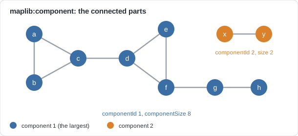
print(m.query("""
SELECT ?node ?id ?size WHERE {
    ?node maplib:component ?c .
    ?c maplib:predicate ex:line ;
       maplib:componentId ?id ;
       maplib:componentSize ?size .
} ORDER BY ?id ?node"""))   # a to h: 1, 8; x and y: 2, 2
The options are on a blank node or a variable (?c above); [ ... ] works as well. Every
predicate below takes the same edge options.
What-ifs: maplib:avoid
maplib:avoid takes nodes out of the graph, with their edges, for this query only. It is a what-if
(open switches, equipment out of service, a closed station) without changing the model. The avoided
nodes have no row:
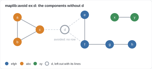
print(m.query("""
SELECT ?node ?id WHERE {
    ?node maplib:component [
        maplib:predicate ex:line ; maplib:avoid ex:d ; maplib:componentId ?id
    ]
} ORDER BY ?id ?node"""))   # e, f, g, h: 1; a, b, c: 2; x, y: 3
maplib:avoid also takes a variable that the group binds, so the nodes to avoid can be found by a
query, e.g. every node marked as open. Put the patterns that find them in a subquery before the
magic predicate:
m.reads(f"@prefix ex: <{EX}> . ex:d ex:open true .", format="turtle")
print(m.query("""
SELECT ?node ?id WHERE {
    { SELECT ?open WHERE { ?open ex:open true } }
    ?node maplib:component [ maplib:predicate ex:line ; maplib:avoid ?open ; maplib:componentId ?id ]
} ORDER BY ?id ?node"""))   # as above
Bridges
A bridge is an edge whose loss splits its component. ?a maplib:bridge ?o gives one row per
bridge, with maplib:object binding the other end and maplib:cutOff the number of nodes on the
smaller side, which is how much the loss would cut off:
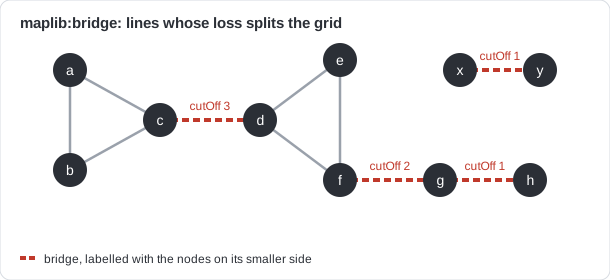
print(m.query("""
SELECT ?a ?b ?cut WHERE {
    ?a maplib:bridge ?o .
    ?o maplib:object ?b ; maplib:predicate ex:line ; maplib:cutOff ?cut .
} ORDER BY DESC(?cut)"""))   # c-d 3, f-g 2, g-h 1, x-y 1
The edges of the triangles are not bridges, as each has a way around it. Parallel edges are not
bridges either. maplib:edgePredicate gives the predicate of the bridge’s edge.
Articulation points
An articulation point is a node whose loss splits its component. maplib:cutOff is the number of
nodes no longer connected to the largest remaining part:
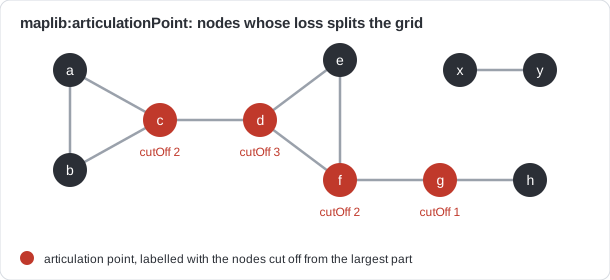
print(m.query("""
SELECT ?n ?cut WHERE {
    ?n maplib:articulationPoint [ maplib:predicate ex:line ; maplib:cutOff ?cut ]
} ORDER BY DESC(?cut)"""))   # d 3, c 2, f 2, g 1
Losing c leaves a, b apart from d to h (2 cut off); losing d leaves a, b, c apart
from e to h (3 cut off).
Edges given by a query: maplib:edgeSource and maplib:edgeTarget
Often the edges of the network are not single triples. A power line connects the substations at its
two ends through terminals and connectivity nodes, for instance. maplib:edgeSource ?a ; maplib:edgeTarget ?b make one edge of every distinct solution of the patterns that bind ?a and
?b, so derived edges need no materialization. Put those patterns in a subquery:
m.reads(f"""
@prefix ex: <{EX}> .
ex:l1 ex:from ex:p ; ex:to ex:q .
ex:l2 ex:from ex:q ; ex:to ex:r .
ex:l3 ex:from ex:q ; ex:to ex:r .
""", format="turtle")
print(m.query("""
SELECT ?line ?a ?b ?cut WHERE {
    { SELECT ?line ?a ?b WHERE { ?line ex:from ?a ; ex:to ?b } }
    ?a maplib:bridge ?o .
    ?o maplib:object ?b ; maplib:edgeSource ?a ; maplib:edgeTarget ?b ; maplib:cutOff ?cut .
}"""))   # l1 from p to q, cutting off 1; l2 and l3 are parallel, so neither is a bridge
The rows keep the other variables of the subquery (?line above), so a bridge comes back with the
line that makes it. A CIM grid’s substation graph, with each line between the substations of its
two terminals:
PREFIX cim: <http://iec.ch/TC57/CIM100#>
PREFIX maplib: <https://datatreehouse.github.io/maplib/vocab#>
SELECT ?line ?s1 ?s2 ?cut WHERE {
    { SELECT DISTINCT ?line ?s1 ?s2 WHERE {
        ?line a cim:ACLineSegment .
        ?t1 cim:Terminal.ConductingEquipment ?line ; cim:Terminal.ConnectivityNode ?n1 .
        ?t2 cim:Terminal.ConductingEquipment ?line ; cim:Terminal.ConnectivityNode ?n2 .
        ?n1 cim:ConnectivityNode.ConnectivityNodeContainer/cim:VoltageLevel.Substation ?s1 .
        ?n2 cim:ConnectivityNode.ConnectivityNodeContainer/cim:VoltageLevel.Substation ?s2 .
        FILTER(STR(?s1) < STR(?s2))   # each line once
    } }
    ?s1 maplib:bridge ?o .
    ?o maplib:object ?s2 ; maplib:edgeSource ?s1 ; maplib:edgeTarget ?s2 ; maplib:cutOff ?cut .
} ORDER BY DESC(?cut)
Every row is an edge, and two rows between the same nodes are parallel edges, which are never
bridges. A pattern that is symmetric in ?a and ?b (like the terminals above) gives each line
twice, once in each direction, so keep one direction with a filter such as
FILTER(STR(?s1) < STR(?s2)); two different lines between the same substations then stay
parallel, as they should. On the Nordic44 test grid this query gives 18 bridges.
The algorithms know nothing of CIM: the grid is only in the query, and the same predicates work on rail nets, pipelines or call graphs.
Counting only some nodes, restricting the rows, and strong components
maplib:countNodestakes nodes (a variable bound by the group, or constants) and makes only them count incomponentSizeandcutOff, e.g. the customers or substations cut off rather than every node of the graph.A subject bound by other patterns of the same block restricts the rows to those nodes. Nodes among them without edges are then components of their own.
maplib:strong truegives the strongly connected components of the directed edges, which is what a cycle check or a dependency analysis needs.
Predicate |
Rows |
Outputs |
|---|---|---|
|
one per node |
|
|
one per bridge (an edge whose loss splits its component), |
|
|
one per node whose loss splits its component |
|
The edge options are those of maplib:shortestPath (maplib:predicate, maplib:inversePredicate,
maplib:anyPredicate, maplib:excludePredicate) or maplib:edgeSource/maplib:edgeTarget;
maplib:avoid and maplib:countNodes take a variable bound by the group (or a subquery before
it) or constants.
Speed and pitfalls
The algorithms run on the cached integer graph of maplib:shortestPath: union-find for
components, Tarjan’s algorithms for strong components, bridges and articulation points, all
without recursion, so deep graphs do not overflow the stack. A grid of ten million triples answers
in well under a second.
Write the patterns that restrict the rows in the same block as the predicate, after a subquery of avoided nodes. A separate block before the subquery is joined with it first, which is a cross product.
Standards and compliance
No W3C or ISO standard defines these algorithms in a query language. SPARQL 1.1 and 1.2 have no graph
algorithms, and ISO GQL and SQL/PGQ leave them to vendor procedures. Other RDF stores also use their
own extensions, such as AnzoGraph’s connected components SERVICE. maplib therefore follows the textbook
definitions (a bridge or an articulation point is an edge or a node whose removal increases the
number of connected components) and is checked against them. The tests in
py_maplib/tests/test_graph_algorithms.py cover the cases above, and
py_maplib/tests/test_graph_algorithm_definitions.py checks maplib on random graphs against the
definitions themselves, by removing every edge and every node in turn. Connected components are also
checked against the validation graphs of the LDBC Graphalytics
benchmark, which defines weakly connected components with reference outputs
(py_maplib/tests/test_ldbc_graphalytics_wcc.py).
Full-text search: maplib:fts EE
Enable the index with IndexingOptions(fts=True) (or create_index), then search with the magic
predicate maplib:fts. Matching is case insensitive, with score 1.0 for a match of the whole
value and 0.75 for a substring match.
m = Model(indexing_options=IndexingOptions(fts=True))      # EE
m.read("data.ttl")
df = m.query("""
PREFIX maplib: <https://datatreehouse.github.io/maplib/vocab#>
SELECT ?subj ?p ?object ?score WHERE {
    ?subj maplib:fts ?fts .
    ?fts maplib:ftsQuery "breaker" ;
         maplib:ftsLimit 10 ;
         maplib:ftsObject ?object ;
         maplib:ftsPredicate ?p ;
         maplib:ftsScore ?score .
}""")
maplib:ftsUniqueSubject true returns each subject once. IndexingOptions(fts_predicates=[...])
limits the index to some predicates. fts_local_names=True also indexes the local names of
subject IRIs, matched with the predicate maplib:ftsLocalName, and fts_iris=True indexes IRIs in the
object position.
GeoSPARQL EE
With IndexingOptions(geo=True), geometry literals (geo:wktLiteral, geo:wkbLiteral,
geo:geoJSONLiteral) are indexed spatially, and the GeoSPARQL functions are available: the simple
features, Egenhofer and RCC8 relations, measurements with units, constructions and serializations,
across coordinate reference systems. Spatial filters and joins use the index. geof:relate, the
query rewrite extension and the aggregates are not supported yet.
m = Model(indexing_options=IndexingOptions(geo=True))      # EE
m.read("features.ttl")
df = m.query("""
PREFIX geo: <http://www.opengis.net/ont/geosparql#>
PREFIX geof: <http://www.opengis.net/def/function/geosparql/>
PREFIX rdfs: <http://www.w3.org/2000/01/rdf-schema#>
SELECT ?l WHERE {
    ?f rdfs:label ?l ; geo:hasGeometry/geo:asWKT ?g .
    FILTER(geof:sfWithin(?g, "POLYGON((1 1, 6 1, 6 6, 1 6, 1 1))"^^geo:wktLiteral))
}""")
10. Insert, update and federation
insert
insert(construct, ...) runs a CONSTRUCT query and adds the triples. It returns the newly added
triples (those not already there) as a dict from predicate IRI to DataFrame. Run the same string
with query first to see what would be added:
m = Model()
m.add_prefixes({"ex": EX})
m.reads(f"<{EX}hawaiian> <{EX}hasIngredient> <{EX}pineapple> .", format="ntriples")

controversial = "CONSTRUCT { ?p a ex:ControversialPizza } WHERE { ?p ex:hasIngredient ex:pineapple }"
print(m.query(controversial)[0])          # inspect
new = m.insert(controversial)             # commit
print(list(new))                          # ['http://www.w3.org/1999/02/22-rdf-syntax-ns#type']
print(m.insert(controversial))            # {}: nothing new
source_graph= is the graph the query reads, and target_graph= the graph the triples go to,
e.g. TRANSIENT_GRAPH. solution_mappings=True returns SolutionMappings. include_graphs,
parameters, max_rows and debug work as for query.
update
update(sparql_update, ...) runs SPARQL 1.1 Update: INSERT DATA, DELETE DATA,
INSERT/DELETE ... WHERE, DELETE WHERE, CLEAR, DROP, ADD/COPY/MOVE and LOAD.
m.update("""
DELETE { ?p ex:hasIngredient ex:pineapple }
INSERT { ?p ex:hasIngredient ex:mango }
WHERE  { ?p ex:hasIngredient ex:pineapple }
""")
m.update("INSERT DATA { GRAPH <urn:g> { ex:margherita a ex:Pizza } }")
m.update("INSERT { GRAPH ?g { ?p ex:inGraph true } } WHERE { GRAPH ?g { ?p a ex:Pizza } }")
print(m.query("SELECT ?p ?i WHERE { ?p ex:hasIngredient ?i }"))
graph=, include_graphs, parameters, max_rows and debug work as for query.
Federation: SERVICE and LOAD
set_federation(...) enables SPARQL 1.1 Federated Query (SERVICE) and LOAD for the queries and
updates of the model, and replaces earlier settings:
m.set_federation(
    allowed_endpoints=["https://query.wikidata.org/sparql", "http://localhost:7878"],  # by URL prefix
    headers={"https://query.wikidata.org": {"User-Agent": "my-app/1.0"}},
    timeout=60.0,
)
df = m.query("""
PREFIX wdt: <http://www.wikidata.org/prop/direct/>
SELECT ?item ?label WHERE {
    VALUES ?item { <http://www.wikidata.org/entity/Q20> }
    SERVICE <https://query.wikidata.org/sparql> {
        ?item <http://www.w3.org/2000/01/rdf-schema#label> ?label FILTER(LANG(?label) = "en")
    }
}""")
A SERVICE pattern runs after the local patterns of its group. The distinct values that the
local patterns bind for the shared variables are sent with it, as VALUES blocks of batch_size rows
(a bind join), so the endpoint only returns matching solutions. SERVICE SILENT gives an empty solution
when the endpoint fails, and SERVICE ?endpoint queries the endpoints the variable is bound to.
With allowed_endpoints=None (the default) any http(s) URL is allowed, and [] allows none.
Other settings: max_rows, concurrency, method ("POST" or "GET"), and bind_join=False to
join locally. arrow and arrow_batch_size control the Arrow format used with maplib endpoints.
LOAD <url> [INTO GRAPH <g>] reads an RDF file from an http(s) URL, object storage, or a file://
URL listed in allowed_endpoints. It needs allow_load=True:
import pathlib

pathlib.Path("extra.ttl").write_text(f"<{EX}x> <{EX}p> <{EX}y> .")
url = pathlib.Path("extra.ttl").resolve().as_uri()
m.set_federation(allowed_endpoints=[url], allow_load=True)
m.update(f"LOAD <{url}> INTO GRAPH <urn:loaded>")
print(m.size("urn:loaded"))   # 1
11. User-defined functions and the query cache
add_udf and list_udfs
add_udf(iri, func, output_type, input_types=None) registers a Python function that SPARQL can
call by its IRI. The function gets a Polars DataFrame with one column per argument, named "0",
"1" and so on. It returns the DataFrame with an added output column, or a Series. output_type
is an RDFType or a datatype IRI:
from maplib import xsd, RDFType

def contains_abc(df: pl.DataFrame) -> pl.DataFrame:
    return df.with_columns(pl.col("0").str.contains("abc").alias("out"))

def shout(df: pl.DataFrame) -> pl.Series:
    return df["0"].str.to_uppercase() + "!"

m = Model()
m.reads(f'<{EX}a> <{EX}s> "xabcx" .\n<{EX}b> <{EX}s> "xyz" .', format="ntriples")
m.add_udf("urn:maplib:containsAbc", contains_abc, xsd.boolean, [xsd.string])
m.add_udf("urn:maplib:shout", shout, RDFType.Literal(xsd.string))
print(m.list_udfs())
print(m.query("""
SELECT ?x ?found ?loud WHERE {
    ?x <http://example.net/ns#s> ?s .
    BIND(<urn:maplib:containsAbc>(?s) AS ?found)
    BIND(<urn:maplib:shout>(?s) AS ?loud)
}"""))
The query cache
set_query_cache keeps the results of query (and of serve EE). A result is kept until a write
changes triples it can read: writes are tracked per graph and predicate, so a write elsewhere
keeps it. It is off by default.
from maplib import QueryCacheOptions

m.set_query_cache(QueryCacheOptions(max_entries=2048, ttl=None))   # or True for the defaults
q = "SELECT ?x WHERE { ?x <http://example.net/ns#s> ?s }"
m.query(q)                          # runs the query
m.query(q)                          # from the cache
print(m.query_cache_stats()["hits"])     # 1
print(m.get_query_cache().max_entries)   # 2048
m.query(q, cache=False)             # bypass it for one query
m.clear_query_cache()               # drop the results, keep the options
m.set_query_cache(False)            # turn it off
QueryCacheOptions(enabled=True, max_entries=1024, max_bytes=256 MiB, max_entry_bytes=16 MiB, ttl=None, min_run_time=0.0, cache_virtualized=False). Queries with parameters or debug, and
queries calling NOW(), RAND(), UUID(), STRUUID(), BNODE() or UDFs, are never cached.
Results over virtualized databases are only kept with cache_virtualized=True, and then a ttl
should be set.
12. Reasoning and validation
infer_rdfs
infer_rdfs(graph=None) applies the RDFS rules 2, 3, 5, 6, 7, 8, 9, 10 and 11 (domain, range,
subproperties and subclasses). The inferred triples go in the transient graph, so they can be
queried but are not written. It returns the number of inferred triples.
m = Model()
m.reads(f"""
@prefix ex: <{EX}> .
@prefix rdfs: <http://www.w3.org/2000/01/rdf-schema#> .
ex:Dog rdfs:subClassOf ex:Animal .
ex:owns rdfs:range ex:Thing .
ex:rex a ex:Dog .
ex:alice ex:owns ex:rex .
""", format="turtle")
print(m.infer_rdfs())
print(m.query("SELECT ?t WHERE { <http://example.net/ns#rex> a ?t }"))   # Dog, Animal, Thing
Datalog: infer EE
infer(rulesets, graph=None, max_iterations=100_000, include_graphs=None, max_rows=100_000_000, debug=False) runs Datalog rules to a fixpoint and adds the inferred triples. With profile=
instead of rulesets, it runs a built-in reasoning profile, see the next section. A rule is
head :- body ., with triple patterns written [subject, predicate, object]:
rules = """
PREFIX ex: <http://example.net/ns#>
[?a, ex:ancestor, ?b] :- [?a, ex:parent, ?b] .
[?a, ex:ancestor, ?c] :- [?a, ex:parent, ?b], [?b, ex:ancestor, ?c] .
[?p, ex:category, "adult"] :- [?p, ex:age, ?age], FILTER(?age >= 18) .
"""
result = m.infer(rules)          # EE; also takes a list of rulesets
Bodies can use FILTER(...), BIND(expr AS ?v) and AGGREGATE(... ON ?group BIND SUM(?x) as ?s).
A ruleset can also consist of SPARQL CONSTRUCT queries, which are run as rules. Prefixes added with
add_prefixes are known in rules. debug=True reports rule bodies that give no triples.
Reasoning profiles: infer(profile=…) EE
infer(profile="owl-rl", graph=None, target_graph=None, include_graphs=None, max_violations=1000, max_rows=100_000_000) materializes the entailments of a built-in reasoning profile with the Datalog
engine. The schema (classes, properties, restrictions and lists) is compiled into rules, which run to
a fixpoint. The profiles are:
"owl-rl": the OWL 2 RL/RDF rules of OWL 2 Profiles: equality, property axioms (inverse, symmetric, transitive, functional, inverse functional, property chains, keys), class expressions (intersection, union, one of, some, all and has value, max (qualified) cardinality 1), class axioms and schema rules. The rules that concludefalseare checked after inference and reported as violations. Not included:x owl:sameAs xfor every term (eq-ref) and the datatype rules dt-type2, dt-eq, dt-diff and dt-not-type."rdfs-plus": a cheaper preset: domain, range, subproperties and subclasses, plusowl:inverseOf, symmetric and transitive properties,owl:equivalentClass,owl:equivalentProperty,owl:sameAsand functional and inverse functional properties. It adds no axiomatic or reflexive triples and checks nothing."rdfs": all the RDFS entailment rules of RDF 1.1 Semantics (rdfD2, rdfs1 to rdfs13) with the RDF and RDFS axiomatic triples, except rdfs4a, rdfs4b and the axiomatic triples that would make every term anrdfs:Resource.
Parameters:
graph: the graph to reason over, the default graph by default.target_graph: where the inferred triples go. By default the transient graph, so they can be queried but are not written. There is one transient graph, shared by all graphs and included in queries by default, so when you reason over several named graphs separately, give each its own target graph. PassDEFAULT_GRAPH(or the graph itself) to add the triples to it. Triples that are already in the graph are not added again.include_graphs: graphs read along with the graph, as with FROM.Noneincludes the transient graph,[]reads only the graph itself and the target graph.max_violations: the most violations reported per rule;0skips the consistency checks.max_rows: the most estimated rows in the result of a rule, to avoid running out of memory.
It returns a ReasoningResult with profile, inferred_triples, consistent, violations (a
list of dicts with rule, message and nodes), violations_truncated, rounds, rules,
rule_executions and seconds.
m = Model()
m.reads("""
@prefix ex: <http://example.org/> .
@prefix owl: <http://www.w3.org/2002/07/owl#> .
ex:partOf a owl:TransitiveProperty ; owl:inverseOf ex:hasPart .
ex:Breaker owl:disjointWith ex:Transformer .
ex:bay1 ex:partOf ex:substation1 . ex:substation1 ex:partOf ex:region1 .
ex:b1 a ex:Breaker, ex:Transformer .
""", format="turtle")
res = m.infer(profile="owl-rl")   # EE
print(res.inferred_triples, res.consistent)   # consistent is False
for v in res.violations:
    print(v["rule"], v["message"])            # cax-dw: ex:b1 is an instance of the disjoint classes ...
print(m.query("SELECT ?x WHERE { <http://example.org/region1> <http://example.org/hasPart> ?x }"))
# bay1 and substation1, through transitivity and the inverse property
Choosing between them: infer_rdfs is in the open-source core. It runs the RDFS rules once each,
in order, as SPARQL inserts, which is fast and enough for typical class and property hierarchies.
infer(profile="rdfs") computes the complete RDFS closure (for example, types from domains of
subproperties found late), with the axiomatic triples, on the Datalog engine. infer(profile="rdfs-plus")
adds the common OWL property axioms and equality without the cost of axiomatic triples or checks;
use it for inverse and transitive properties in models such as CIM. Use infer(profile="owl-rl") for
class expressions, property chains, keys and consistency checks.
Inferring or asserting owl:sameAs is costly for large groups of equal resources, because the
triples of every member are copied to the others.
SHACL: validate EE
validate(...) validates a graph against SHACL Core and SHACL-SPARQL shapes, evaluating shapes in
parallel, and runs SHACL rules (sh:rule):
m = Model()
m.reads("""
@prefix sh: <http://www.w3.org/ns/shacl#> .
@prefix ex: <http://example.org/> .
ex:PersonShape a sh:NodeShape ; sh:targetClass ex:Person ;
    sh:property [ sh:path ex:name ; sh:minCount 1 ; sh:message "Missing name"@en ] .
""", format="turtle", graph="urn:shapes")
m.reads("@prefix ex: <http://example.org/> . ex:alice a ex:Person .", format="turtle")

report = m.validate(shape_graph="urn:shapes", report_graph="urn:report")   # EE
print(report.conforms)          # False
print(report.results())         # one row per result; message is a list of strings
print(report.shape_targets)     # targets per shape and constraint
print(report.performance)
Options: data_graph, report_graph ("" (the default) writes no report graph, None writes it
to the default graph), inferences_graph (for sh:rule results, otherwise the transient graph),
include_details=True (then report.details()), include_conforms, only_shapes /
deactivate_shapes, dry_run (only find the targets), max_rows, serial, max_iterations and
debug_rules (with report.rule_log).
13. Virtualization EE
Virtualization leaves large time series in the database that holds them. The graph describes the time series, and the parts of a SPARQL query that read their data points are translated to the database’s query language. Filters, grouping and ordering are pushed down where possible.
VirtualizedDatabase and add_virtualization
Each time series in the graph has chrontext:hasResource (the name of a resource) and
chrontext:hasExternalId (its id in the database). A resource has a template describing its
rows, which must have an id parameter:
from maplib import Model, VirtualizedDatabase, Template, Parameter, Variable, RDFType, Triple, Prefix, xsd
from maplib.virtualization import DuckDBDatabase

ct = Prefix("https://github.com/DataTreehouse/chrontext#")
id_, ts, value, dp = Variable("id"), Variable("timestamp"), Variable("value"), Variable("dp")
readings = Template(
    iri=ct.suf("readings"),
    parameters=[
        Parameter(id_, rdf_type=RDFType.Literal(xsd.string)),
        Parameter(ts, rdf_type=RDFType.Literal(xsd.dateTime)),
        Parameter(value, rdf_type=RDFType.Literal(xsd.double)),
    ],
    instances=[
        Triple(id_, ct.suf("hasDataPoint"), dp),     # name the data point with a variable, not a blank node
        Triple(dp, ct.suf("hasValue"), value),
        Triple(dp, ct.suf("hasTimestamp"), ts),
    ],
)
vdb = VirtualizedDatabase(
    DuckDBDatabase(database="readings.duckdb"),
    resource_sql_map={"readings": "SELECT sensor_id AS id, ts AS timestamp, value FROM readings"},
)
m = Model()
m.reads("""
@prefix ct: <https://github.com/DataTreehouse/chrontext#> .
@prefix ex: <http://example.net/ns#> .
ex:pump1 ex:hasSensor ex:s1 . ex:s1 ct:hasTimeseries ex:ts1 .
ex:ts1 ct:hasResource "readings" ; ct:hasExternalId "sensor-1" .
""", format="turtle")
m.add_virtualization(vdb, resources={"readings": readings})      # EE
df = m.query("""
PREFIX ct: <https://github.com/DataTreehouse/chrontext#>
PREFIX ex: <http://example.net/ns#>
PREFIX xsd: <http://www.w3.org/2001/XMLSchema#>
SELECT ?pump (AVG(?v) AS ?avg) WHERE {
    ?pump ex:hasSensor/ct:hasTimeseries ?t .
    ?t ct:hasDataPoint ?p . ?p ct:hasTimestamp ?at ; ct:hasValue ?v .
    FILTER(?at >= "2024-01-01T00:00:00Z"^^xsd:dateTime)
} GROUP BY ?pump""")
VirtualizedDatabase(database, resource_sql_map=None, sql_dialect=None, pushdowns=None): any object with aquery(sql) -> pl.DataFramemethod works as the database, given asql_dialect("duckdb","postgres","snowflake","bigquery","databricks"or anSQLDialect). The SQL of a resource can be a string, an SQLAlchemyTableorSelect. Withoutresource_sql_map, thequerymethod gets theVirtualizedQueryitself (maplib.vq) to translate.pushdownschooses among"value_conditions","group_by"and"ordering".add_virtualizationcan be called several times to query several databases together. Joins between time series are only pushed down within one database.VirtualizedDatabase.Cognite(client, resource_cognite_map=None)reads time series from Cognite Data Fusion.
maplib.virtualization
Ready-made databases, which know their dialect: DuckDBDatabase, SnowflakeDatabase,
BigQueryDatabase, DatabricksDatabase, TimescaleDatabase, InfluxDBDatabase (InfluxDB 3, SQL),
InfluxDB2Database (InfluxDB 2 / 1.8, Flux; resources are measurements),
FabricLakehouseDatabase, FabricDatabase (Fabric Warehouse, T-SQL) and KustoDatabase (Azure
Data Explorer and Fabric Eventhouses; resources are KQL expressions). SQLDatabase is the base class
for your own. The dialect classes (PostgresDialect, DuckDBDialect, SnowflakeDialect, …),
translate_sql and translate_kql let you customise or inspect the generated queries.
maplib.opcua.OPCUAHistoryDatabase(endpoint, ...) reads OPC UA Historical Access, with node ids
such as ns=2;s=ts1 as external ids.
from maplib.virtualization import SnowflakeDatabase
from maplib.opcua import OPCUAHistoryDatabase

snow = VirtualizedDatabase(
    SnowflakeDatabase(account="...", user="...", warehouse="...", database="...", schema="..."),
    resource_sql_map={"readings": "SELECT sensor_id AS id, ts AS timestamp, value FROM readings"},
)
opcua = VirtualizedDatabase(database=OPCUAHistoryDatabase("opc.tcp://plant:4840/"))
m.add_virtualization(snow, resources={"readings": readings})
m.add_virtualization(opcua, resources={"history": readings})
Industrial sources: map_cdf, map_osipi, map_pi_points, map_insights_hub and maplib.ip21
These read a source’s own asset model into the graph and virtualize its time series in one call. Their docstrings describe the vocabulary each one produces.
from cognite.client import CogniteClient
m.map_cdf(CogniteClient(), data_models=[("my_space", "MyModel", "v1")])     # Cognite Data Fusion

m.map_osipi("https://myserver/piwebapi", asset_database="\\\\MyAFServer\\MyDatabase",
            username="me", password="...")                                  # PI Asset Framework
m.map_pi_points("https://myserver/piwebapi", data_server="MyPIServer", name_filter="FIC*",
                username="me", password="...")                             # PI Data Archive tags
m.map_insights_hub("gateway.eu1.mindsphere.io", "mytenant",
                   client_id="mytenant-svc", client_secret="...")           # Siemens Insights Hub

from maplib.ip21 import map_ip21
map_ip21(m, "https://ip21server/ProcessData/AtProcessDataREST.dll", "IP21",
         tag_filter="FIC*", default_start_time="2024-01-01T00:00:00Z")      # AspenTech IP.21
Their data points are queried like any other virtualized time series:
df = m.query("""
PREFIX osipi: <urn:maplib_osipi:>
PREFIX chrontext: <https://github.com/DataTreehouse/chrontext#>
PREFIX xsd: <http://www.w3.org/2001/XMLSchema#>
SELECT ?tag ?bucket (AVG(?v) AS ?avg) WHERE {
    ?p a osipi:Point ; osipi:name ?tag ; chrontext:hasDataPoint ?dp .
    ?dp chrontext:hasTimestamp ?t ; chrontext:hasValue ?v .
    BIND(chrontext:FloorDateTimeToSecondsInterval(?t, 3600) AS ?bucket)
    FILTER(?t >= "2024-01-01T00:00:00Z"^^xsd:dateTime && ?t < "2024-01-02T00:00:00Z"^^xsd:dateTime)
} GROUP BY ?tag ?bucket""")
Grouping by chrontext:FloorDateTimeToSecondsInterval with MIN, MAX, SUM, COUNT or AVG is read
from the source’s own aggregates where it has them. A query without a lower bound on the timestamp
fails unless default_start_time is set.
14. Configuration, serving and model management
maplib.config
maplib.config keeps a model’s configuration as triples in its own named graph,
maplib.config.CONFIG_GRAPH, so the configuration is written, serialized and served with the model.
apply_config(m) applies it: it creates the indexes, sets the query cache and connects the
virtualizations. Secrets are never stored: a secret names the environment variable that holds it.
CONFIG_GRAPH.md documents the vocabulary.
from maplib.config import (
    CONFIG_GRAPH, IndexingConfig, QueryCacheConfig,
    write_indexing, read_indexing, write_query_cache, read_query_cache, remove_query_cache,
    apply_query_cache, apply_config,
)

m = Model()
write_query_cache(m, QueryCacheConfig(max_entries=2048, ttl=300.0))
write_indexing(m, IndexingConfig(object_sort_some=["http://example.net/ns#serialNumber"]))
print(read_query_cache(m), read_indexing(m))
m.write("model.trig", format="trig")      # the config graph is in the file

m2 = Model()
m2.read("model.trig")
apply_config(m2)                          # sets the cache and creates the indexes
print(m2.get_query_cache().max_entries)   # 2048
Virtualizations EE are configured the same way:
from maplib.config import VirtualizationConfig, VirtualizationResource, write_virtualization, read_virtualizations

write_virtualization(m, VirtualizationConfig(
    iri="urn:maplib:config:virtualization:readings",
    database="snowflake",                  # one of maplib.config.DATABASES
    parameters={"account": "acme", "user": "maplib", "warehouse": "wh", "database": "meters", "schema": "public"},
    secrets={"password": "SNOWFLAKE_PASSWORD"},          # read from the environment by apply_config
    resources=[VirtualizationResource(
        name="readings",
        sql="SELECT id, ts AS timestamp, value FROM readings",
        template=READINGS_TEMPLATE,                     # a stOTTR document or a template IRI
        properties={"http://iec.ch/TC57/2013/CIM-schema-cim16#Measurement.unitSymbol":
                    "http://iec.ch/TC57/2013/CIM-schema-cim16#UnitSymbol.W"},
    )],
))
applied = apply_config(m)                 # EE; apply_config(m, environ={...}) for other secret sources
Other functions: remove_virtualization, read_virtualizations, apply_virtualization,
apply_properties (writes the static resource properties without connecting) and probe(config),
which checks a configuration against the database without changing a model.
serve EE
serve(...) serves the live model over the SPARQL 1.1 Protocol (/sparql, /query, /update,
/store), the Arrow API over HTTP (/arrow/...) and Arrow Flight, in the background. Queries see
changes made from Python, and the other way round.
import pyarrow.flight

server = m.serve(port=7878, flight_port=7879, allow_update=True, auth_token="secret")   # EE
print(server.url)            # http://127.0.0.1:7878/sparql
df = Model().query("SELECT * WHERE { ?s ?p ?o } LIMIT 5", endpoint=server.url, endpoint_token="secret")
client = pyarrow.flight.connect(server.flight_url)
server.stop()

with m.serve(port=0, flight_port=None) as server:   # stops on exit
    ...
Options include host (use "0.0.0.0" with auth_token), cors_origins, graph and
include_graphs, max_rows, max_request_bytes, arrow_compression, query_log_size (served at
GET /query-log), static_dir/static_path/static_vars for a web app, query_cache,
service_endpoints and allow_load (SERVICE and LOAD are refused unless listed), and block=True.
explore EE
explore() runs the Model portal, a browser UI for browsing, searching and querying the model.
server = m.explore(port=8000)     # EE
print(server.url)                 # open it in a browser
print(server.sparql_url)          # the portal's SPARQL endpoint
server.stop()
The module-level maplib.explore(m, ...) is deprecated; use m.explore().
Indexes and compaction
from maplib import IndexingOptions, IRI

m = Model()
m.reads(f'<{EX}a> <{EX}serialNumber> "123" .', format="ntriples")
m.create_index(IndexingOptions(object_sort_some=[IRI(EX + "serialNumber")]))
m.compact()     # merge the segments that accumulate from repeated additions
create_index sets the indexing options and builds the indexes for the triples already in the
model, dropping object indexes that are no longer chosen. Full-text and geo indexes are EE.
compact merges the stored segments of each predicate into one sorted segment. serialize
also compacts the model.
Introspection
print(m.size())                                   # triples in the default graph
print(m.get_predicate_iris())                     # [IRI(http://example.net/ns#serialNumber)]
tables = m.get_predicate(IRI(EX + "serialNumber"))
print(tables[0].mappings, tables[0].rdf_types)    # the stored tables, as SolutionMappings (columns subject, object)
print(m.list_udfs(), len(m.get_templates()))
print(maplib.__version__)
get_predicate_iris and get_predicate take graph= and include_graphs=.
Threads
A Model can be shared between threads. Reads (query, query_external, write, writes,
write_bytes, size, get_predicate, get_predicate_iris, get_templates and list_udfs) run
at the same time. Changes take an exclusive lock and wait for running reads. Queries release the
GIL while they run, so other Python threads keep working.
from concurrent.futures import ThreadPoolExecutor

with ThreadPoolExecutor(4) as pool:
    sizes = list(pool.map(lambda _: m.query("SELECT * WHERE { ?s ?p ?o }").height, range(8)))
print(sizes)
Errors
Most errors raise maplib.MaplibException, and invalid arguments raise
maplib.FunctionArgumentException. Syntax errors in SPARQL, Datalog and stOTTR show the
offending source with a hint:
from maplib import MaplibException

try:
    m.query("SELEC ?x WHERE { ?x ?p ?o }")
except MaplibException as e:
    print(e)
# SPARQL parsing error: SPARQL syntax error at line 1, column 1: unexpected `SELEC`
#   |
# 1 | SELEC ?x WHERE { ?x ?p ?o }
#   | ^^^^^
#   ...
#   = help: did you mean `SELECT`?
Enterprise features called in the open-source build panic with “Contact Data Treehouse to try”
(a pyo3_runtime.PanicException, which derives from BaseException, not Exception), or raise
NotImplementedError.